Parallel Preconditioned Conjugate Gradients
CS267 Fall 2002 – Assignment 3
Rabin K. Patra, Sergiu Nedevschi, Sukun Kim
Source code:
1. Introduction
The purpose of this assignment is solving linear system Ax=b quickly. There are two major approaches: the Conjugate Gradient algorithm and Sparse Matrix algorithms. We will be concentrating on the Conjugate Gradient method and efficient parallel implementations of the same.
(1) Conjugate gradient algorithm.
To make conjugate gradient algorithm faster, preconditioning is used ([1]). The preconditioning matrix M is an essential factor in performance. As MAMT gets closer to I, performance gets better.
In the Jacobi method, for a given A, diagonal blocks B1, B2, …, Bn are chosen. And their Cholesky factors, C1, C2, …, Cn are computed. Preconditioning matrix M is a collection of these Cholesky factors ([2]). Since Cholesky factor is used, solving Mx=b is easy. Moreover, blocked structure of M enables parallelization of solving Mx=b. We did not change the preconditioning matrix M. We tried to reorder rows and columns of A.
In SSOR, A is used as preconditioning matrix M. However since this is not appropriate for parallelization, we did not use SSOR in parallel implementation.
(2) Parallelism
UPC and Titanium codes are given. UPC ([3]) did not work on Millennium or Seaborg. More functionality and flexibility were given by MPI ([4]) than Titanium ([5]), and we felt more comfortable with MPI. Therefore, we used MPI for parallel implementation.
2. Serial implementation
For serial implementation, we just test the given code.
For Jacobi method, the block size is 50.
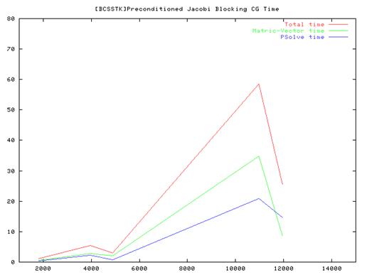
Conclusion:
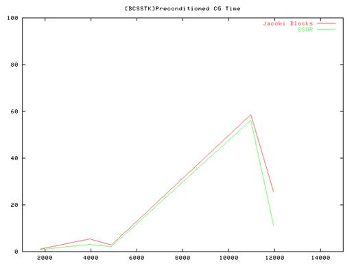
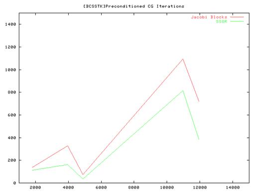
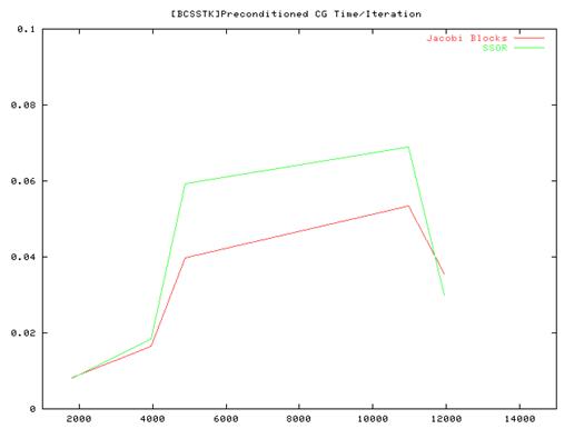
- From the performance results of the serial implementation of the CG algorithm we found that the Vanilla code(without preconditioning) ran very slow compared to the Jacobi and SSOR implementations and we some times did not even converge. So we have plotted results for the Jacobi and SSOR variants of the algorithm.
- Also the amount of time taken for convergence is not strictly related to the matrix size – the number of elements in the sparse matrix structure as well as their layout influences the total time and the no of iterations. This is especially true for the methods that we used which rely on the fact that most of elements are distributed close to the main diagonal of the matrix.
3. Parallel implementation using MPI
Background:
From the performance of the serial code for solving 'Ax=b' - it was clear that the Jacobi and SSOR preconditioning methods were far superior compared to the Vanilla (no preconditioning).
An analysis of both the Jacobi and the SSOR algorithms shows that though the SSOR algorithm is better in terms of no of iterations and the total computation time, the Jacobi method is easier to parallelize. It divides the matrix into blocks which are factorized using Cholesky factorization. This lends itself naturally to a parallel model where blocks are divided among the processors. The other operations of matrix-vector multiplication and the inner product can also be parallelized.
The UPC implementation posted on the homework page was not feasible as neither Millennium nor Seaborg supported the UPC library. The alternatives were MPI and Titanium and we chose MPI as it is more versatile.
The MPI implementation:
- The rows of the original matrix are equally divided among the processors. Each processor then divides its own rows into blocks according to the Jacobi method. Each of these blocks can be handled independently and Cholesky factorization is applied to these blocks.
- The main loop of the CG algorithm involves matrix-vector multiplication of the A matrix with the p vector and this can be parallelized easily by distributing the p vector to all the processors. Each processor multiplies the p vector with its own rows and the result vector is stored.
- The inner product operation is used many times in the main loop and it can also be parallelized. Each processor computes the local inner product for the rows it owns and these local sums are then added using the MPI_Reduce operation to get the final result.
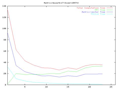
Results: We used matrices from the Matrix Market site for testing the MPI implementation. We tested matrices from two classes of problems and we chose only the reasonably big matrices.
BCS: Structural Engineering Matrices
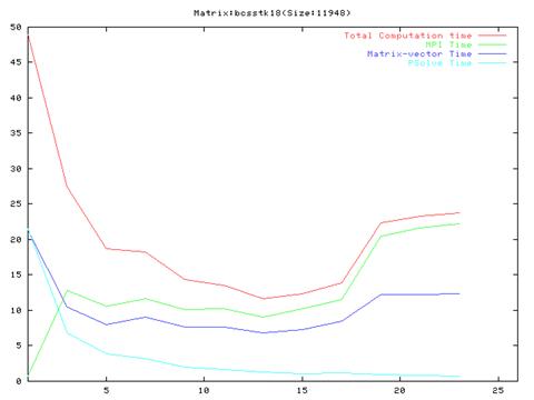
Matrix bcsstk18(759 iterations)

Matrix bcsstk16(75 iterations)
CYLSHELL: Finite element analysis of cylindrical shells
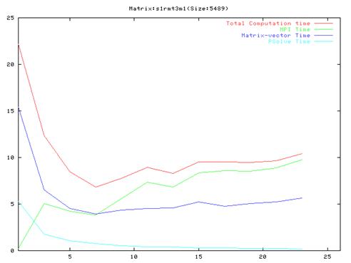
Matrix s1rmt3m1(425 iterations)

Matrix s1rmq4m1(430 iterations)
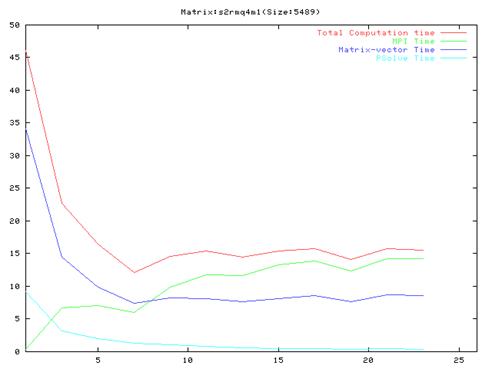
Matrix s2rmq4m1(650 iterations)
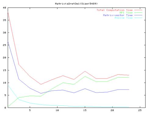
Matrix s2rmt3m1(670 iterations)
Conclusion:
- As evident from the graphs, though results are much better compared to the serial implementation, they do not scale very well and the optimal performance occurs are around 10 processors.
- Also, it is clear from the graphs that the MPI communication time is a large fraction of the total computation time. This is because of the number of MPI operation which we have to do in each iteration of the algorithm. We also found out that the order of the operations in the main loop cannot be changed a lot because of dependencies between the different steps.
4. Fill-reducing using METIS
METIS ([6]) contains a library for fill-reducing reordering routines. This library reorders rows and columns of matrix A so that result matrix A has smaller number of fill elements when Cholesky factorized. We tried this method but the performance degraded. There are two main reasons for this phenomenon, we think. First, we Cholesky-factorize diagonal blocks of matrix not the whole matrix. So this reordering does not guarantee reduced fill in blocked Cholesky factors. Second, this algorithm increases the bandwidth of the given matrix. Since conditioning matrix M contains only diagonal part, wider bandwidth of A makes MAMT farther from I, resulting in worse performance.
5. Narrowing bandwidth
We thought narrowing
bandwidth will make MAMT close to I, and
will give better performance. We tried to find library for Reverse Cuthill-McKee Algorithm ([7]).
To this end, we implemented our
own Reverse Cuthill Mckee
algorithm – which involves Bread First search of the sparse matrix graph giving
us the ordering for the elements(permutation).
Applying this permutation on the original graph gives us the modified sparse
matrix. A key point in the algorithm is to select a good starting point to
start the BFS, and we implemented a heuristic for doing that as proposed in ([7]).
Results:
The CG algorithm does not
always converge after applying the Reverse Cuthill-Mckee
transformation – and sometimes it produces the wrong solution.
|
Matrix |
Size |
Elements |
Initial BW |
Final BW |
Converged? |
Initial iterations |
Final iterations |
|
Nos1 |
237 |
627 |
4 |
4 |
Yes |
30 |
15 |
|
Gr_30_30 |
900 |
4322 |
31 |
59 |
Yes |
21 |
44 |
|
S3rmt3m3 |
5357 |
207695 |
5302 |
212 |
No |
- |
- |
|
1138_bus |
1138 |
4054 |
1030 |
131 |
No |
- |
- |
Conclusion:
- Finding the optimal bandwidth in a matrix is
NP-complete, so we have to use an heuristic
algorithm and as a result we do not always decrease the bandwidth of the
matrix.
- From the fact that the CG algorithm does not
always converge after this re-ordering, we have the suspicion that
permutation of a matrix does not preserve the positive-definiteness
property though it still remains symmetric. But we have not been able to
prove this rigorously and this can be a subject of study.
6. Reference
[1] Ian Sobey. Conjugate Gradient Algorithm. http://www.sjc.ox.ac.uk/scr/sobey/iblt/chapter1/notes/node20.html
[2] Department of Computer Sciences, The University of Texas at Austin. Cholesky Factorization. http://www.cs.utexas.edu/users/plapack/icpp98/node2.html
[3] The High Performance Computing Laboratory, The George Washington University. Unified Parallel C. http://upc.gwu.edu/
[4] MPI Forum. Message Passing Interface. http://www.mpi-forum.org/
[5] Computer Science Division, University of California at Berkeley. Titanium. http://titanium.cs.berkeley.edu/
[6] George Karypis. METIS. http://www-users.cs.umn.edu/~karypis/metis/index.html
[7] Dale Olesky. The Reverse Cuthill-McKee Algorithm. http://www.csc.uvic.ca/~dolesky/csc449-540/1.5-1.6c.pdf