Structure Monitoring using
Wireless Sensor Networks
CS294-1 Deeply Embedded Network Systems
Abstract
Structure monitoring brings new challenges to wireless
sensor network: high-fidelity sampling, collecting large volume of data, and
sophisticated signal processing. New accelerometer board measures tens of
μG acceleration. High frequency sampling is enabled by new component of
David Gay. With new component, up to 6.67KHz sampling is possible with jitter
less than 10μs. Large-scale Reliable Transfer (LRX) component collects
data at the expense of 15% penalty of channel utilization for no data loss. To
overcome low signal-to-noise ratio, analog low-pass filter is used, and
multiple digital data are averaged. Structure monitoring is a driving force for
extending capability of wireless sensor networks system.
- Introduction
Wireless sensor network enables low-cost sensing of
environment. Many applications using wireless sensor networks have low duty
cycle and low power consumption. However the ability of wireless sensor
networks can be extended in reverse way. Enhanced TinyOS, and new components
opened possibility for more aggressive applications. Structure monitoring is
one example of such applications.
To monitor a structure (e.g. bridge, building), we
measure behavior (e.g. vibration, displacement) of structure, and analyze
health of the structure based on measured data. Figure
1 shows overall system. Each component can have
multiple subcomponents. In our case, sensor is accelerometer which will be
discussed in Section 2, and analog processing has low-pass filter (Section 6.)
Digital processing includes averaging (Section 6), data collection (Section 5),
and system identification (Section 6). Low-jitter control contains
high-frequency sampling (Section 4). There are more sub-components to be added
in the future: time synchronization in low-jitter control, calibration and
digital filtering in digital processing.
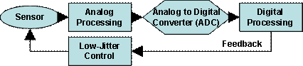
Figure 1 Overall System
Here we present challenges, findings, and our
experience in structure monitoring using wireless sensor networks. Rather than
focusing on one single component, this paper overview overall system and issues
in each component.
- Related Work
Habitat monitoring is a leading application of
wireless sensor network. And it is an example application with low duty cycle.
ZebraNet [1] uses PDA-level device with 802.11b wireless network.
For structure monitoring, there are tremendous
amount of research using conventional wired way. GPS was used combined with
wired data collection [3, 4], however at a high cost. There is an approach
using wireless network for data collection [5], which has great advantage over
wired network. However, it uses large hardware platform (in terms of size,
power, and cost) which diminishes benefit of wireless approach. [6] uses
low-cost device and wireless network, but it is more like conceptual test, and
fidelity is not sufficient for real deployment. We begins with high fidelity
sampling in the following section.
- Data Acquisition
Data acquisition is composed of mainly two parts:
data sampling, and data collection. Structure monitoring requires high fidelity
data sampling. Accurate, high frequency sampling, and low jitter are main
requirement for high quality sample. Accuracy is discussed in this section, and
high frequency sampling with low jitter will be covered in Section 4. And data
collection will be discussed in Section 5.
In structure monitoring, acceleration signal is
very week. Detecting even moderate earthquake requires to measure 500μG
acceleration. Sensitivity and accuracy of accelerometer is crucial, so we put
significant portion of effort to accelerometer board. New accelerometer board
was designed by as shown in Figure 2.
3.1.
Accelerometers
It has two kinds of accelerometers: ADXL 202E, Silicon
Designs 1221L. Table 1 shows characteristics of each accelerometer combined
with entire system. Accelerometer board contains 1 of ADXL 202E, and 2 of
Silicon Designs 1221L, and 4 16bit analog to digital converter (ADC). There are
two channels for ADXL 202E, and two channels for Silicon Designs 1221L with
same orientation. One is parallel to gravity, and the other is vertical to
gravity. Initially both accelerometers had range of -2G ~ 2G, but for better
sensitivity, range of Silicon Designs 1221L is change to -0.1G ~ 0.1G. Channel
with axis parallel to gravity has 1G offset to compensate for offset by
gravity. It also contains one temperature sensor (reason will be explained
later). New version of
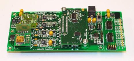
Figure 2 Accelerometer Board
Table 1 Two Accelerometers Combined with System
|
|
ADXL
202E |
Silicon
Designs 1221L |
|
Type |
MEMS |
MEMS |
|
Number
of axis |
2 |
1 |
|
Range |
-2G
~ 2G |
-0.1G
~ 0.1G |
|
System
noise floor |
200(μG/√Hz) |
30(μG/√Hz) |
|
Price |
$10 |
$150 |
3.2.
Noise Floor Test and Shaking Table Test
To see static characteristic of accelerometers, accelerometer
board was put to quiet place (from vibration and sound) with constant
temperature. This test shows noise floor which is shown in Table 1. For Silicon Designs 1221L, range was -0.1G ~ 0.3G.
Then to see dynamic behavior of accelerometers, we performed shaking table test
with constant temperature. Even though test site was not completely free from
vibration and sound noise, it was quiet enough for a dynamic range of shaking
table to dominate noise. Results are shown in Figure 3. Left figure is result of ADXL 202E, right one is
result of Silicon Designs 1221L, and driving frequency is 0.5Hz. Data are read
from both channels at the same time. For this test, channel for Silicon Designs
1221L had range of -2G ~ 2G.
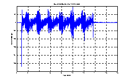

Figure 3 Shake
Table Test (0.5Hz)
We can see Silicon Designs 1221L shows cleaner
shape in both static situation and dynamic situation. Figure
4 show another experiment on shaking table. Here
frequency increases while displacement remains constant. When movement gets
rigorous, Silicon Designs 1221L does not properly read it. It seems like
Silicon Designs 1221L has larger damping factor than ADXL 202E.
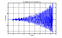
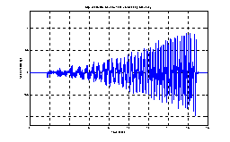
Figure 4 Shaking Table Test (Increasing
frequency with same displacement)
3.3.
Tilting Test and Vault Test
To measure linearity of accelerometer value, we performed
tilting test with help of Bob Uhrhammer. By changing tilting degree of
accelerometer, we can obtain line showing acceleration value read versus real
acceleration. Only channel vertical to gravity is measured of Silicon Designs
1221L. For this test, range was -0.1G ~ 0.3G. Deviation from minimum mean
square error line is within 60μG
For a better noise floor test, we went to a vault
in Lawrence Berkeley Laboratory. Figure 5 shows how quiet inside of vault is compared to normal
office environment. And it also shows reference reading from very sophisticated
accelerometer in the vault, which is used for seismic research. System with
Silicon Designs 1221L shows 20dB higher noise level. Figure
6 shows time plot of acceleration in vault and office
environment for 30 minute period. Red line shows noise in normal office
environment. We can see noise from machines, which is also visible in Figure 5. Blue line shows acceleration readings from vault.
Drift is observed in this case. On test day, it was cold, and inside of vault
was hot by lights. We put accelerometer in a vault, and immediately started
sampling. So accelerometer board was under drastic change in temperature. Drift
is almost 10mG which is significant compared to noise floor, and sensitivity.
More discussion on temperature will follow in Section 8 Future work.
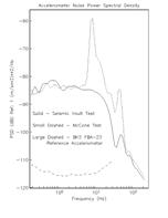
Figure 5 Noise Power Spectral Density
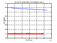
Figure 6 Time Plot of Acceleration
4.
High-frequency Sampling
Characteristic vibration frequency of a structure
is usually around 10Hz rage. However by Nyquist theorem, sampling rate should
be at least twice of that. Moreover, to reduce effect of noise averaging is
used, and sampling rate is multiplied by the number of samples averaged. All
these factors increase sampling rate to KHz level. Structure monitoring
requires regular sampling with uniform interval, and jitter becomes harder
problem as sampling rate gets higher. There are two kinds of sources to jitter,
and they are shown in Figure 7. Temporal jitter occurs inside of node, because
actual sampling does not occur at uniform interval. So even with only one node,
temporal jitter happens. Spatial jitter happens because of variation in
hardware, and imperfect time synchronization. Even if two nodes agree to sample
at time T, this T occurs at different absolute times for those two nodes.
Spatial jitter occurs only when there are more than one node. Here only temporal
jitter is considered. Spatial jitter will be discussed in Section 8 Future
Work.
David Gay wrote a new component
HighFrequencySampling, which enables KHz range sampling. This new component is
introduced in Section 4.1, jitter test result is shown in Section 4.2, and
theoretical jitter analysis follows in Section 4.3.
Figure 7 Sources of Jitter
4.1.
HighFrequencySampling component
This component is written by David Gay for sampling
at KHz level frequency. Pre-existing components can sample only up to 200Hz.
There are two major sub-components which enable high frequency sampling.
MicroTimer is a new timer component which directly
accesses hardware timer, and does not provide multiple abstract timers. This is
very simple and quick to process timer events. BufferLog is a flash memory
writer. It has two buffers. One is filled up by upper layer application while
the other buffer is written to flash memory as a background task. Those two
components (MicroTimer, BufferLog) have minimum amount and length of atomic
section, which blocks other operation and could introduce queue overflow.
With HighFrequencySampling component, 6.67KHz
sampling is achieved. With averaging 16 samples, 1KHz is achieved, which means
16KHz of sampling.
4.2.
Jitter Test
We tested jitter of HighFrequencySampling
component. Instead of storing acceleration value, time is recorded so that we
can measure jitter. Figure 8 shows jitter as time goes. There are two sections:
plain section, spiky section, even though at 6.67KHz this separation is not
clear. These two sections constitute one epoch. It takes epoch period of time
to fill up buffer. During spiky period, buffer is written to flash memory as a
background task. At 1KHz, only small portion of sampling is affected by flash
memory write. At 6.67KHz, flash memory write takes too much portion of time to
fill up buffer, most of sampling are affected by flash memory write. Looking at
5KHz case, even at 6.67KHz flash memory write should not affect that many sampling.
However, overhead of sampling itself seems to have some effect.
There is another thing interesting. At plain
section, there is a constant delay for every sampling. This delay is wake up time
of CPU. When CPU is idle, it enters a sleeping mode. And it takes 4 cycles to
recover. Since there is a function call to record time, actually it takes 5
cycles here. Since CPU runs at 8MHz, this wakeup time is equal to 625ns.
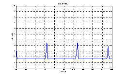
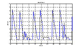
Figure 8 Jitter in Time Line (1KHz, 5KHz, 6.67KHz respectively)
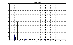
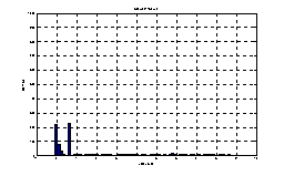
Figure 9 Histogram of Jitter (1KHz, 5KHz, 6.67KHz respectively)
Figure 9 shows distribution of jitter values (histogram). We can see a peak at 625ns, which is wakeup time. Except this peak, frequency of jitter is largest near 0μs, and gradually decreases as jitter value increases. And jitter values are within 10μs. Next section analyzes this phenomenon.
4.3.
Jitter Analysis
Figure 10 shows interaction of sampling and other job (flash
memory write). Timer event for sampling occurs regularly with uniform interval.
However to be serviced in CPU, CPU should finish non-preemptible portion (in
TinyOS, atomic section). Then CPU handles events in event queue which came
before timer event. Then finally timer event for sampling is handled. For our
case, event queue is not likely filled with other waiting events, so this
possibility is not considered here. Then the length of atomic section in
execution determines jitter.
Let T(i) be execution time of atomic section i, and
let X(i) be a random variable uniformly distributed in [0, T(i)]. And let C be
context switch time. Assume that the probability of timer event occurring at
any point in atomic section i is same, then jitter will follow C+X(i). Figure 11 shows this jitter model, where F(i) is frequency of
occurrence of atomic section i.
Since jitter distribution of every atomic section
begins from C, the frequency is highest near C and decreases as moving farther.
And frequency drop at C+T(i) by F(i), since atomic section i will not have any
distribution beyond C+T(i).
Actually there is a peak at C, because when program
is in preemptible section, it will immediately service timer event after
context switch time C.
Figure 10 Occurrence of Jitter

Figure 11 Jitter Model
Test result matches quite well with theoretical
model here. And we can also notice that context switch time C is 0, which means
timer event is handled immediately if program is not in atomic section. There
is one bad news. Worst case jitter is determined by the longest atomic section
of the entire system. So even if we have good component at low layer, if upper
application layer is not well written, system will suffer long worst case
jitter.
High frequency sampling with high accuracy produces
a large amount of data. This large amount of data can not be collected at real
time through wireless communication. So we store data to flash first. And after
sampling enough data, collection starts, and data in flash memory are
transferred. Transferring large amount of data is another challenge. Next
Section explains how we transfer huge volume of data efficiently.
5.
Large-scale Reliable Data Transfer
As we sample at high frequency with large number of
nodes, the amount of data gets large quickly. Let us assume each node store 4Byte
of data and 4Byte of time stamp at 100Hz. And assume there are 100 nodes, radio
throughput is 1.2KB/s, and data is collected to one base station. If
acceleration data worthy 5 minutes is collected, each node will transfer
240,000Bytes. 100 nodes will transfer 24,000,000Bytes. Since the end link to
base station is a bottleneck, it will take more than 5 hours. We can see
bandwidth is narrow compared to aggressive data sampling. Even if we alleviate
this problem using multi-channel or multi-tier network, still we will be in
short of bandwidth.
Moreover, we need to transfer data reliably. We
will be able to overcome some packet losses using data processing, but at
current stage we do not assume this technique.
These needs lead to efficient large-scale reliable
data transfer. Right now RAM to RAM transfer is implemented as a building
block. Multi-hop flash memory to flash memory transfer will be discussed in
Section 8 Future Work.
5.1.
Protocol
Large-scale Reliable Transfer (LRX) component
assumes that data resides in RAM. Upper layer should handle non-volatile
storage. LRX transfers one data cluster, which is composed of several blocks.
One block fits into one packet, so the number of blocks is equal to window size.
Each data cluster has a data description. After looking at data description,
receiver may deny data (receiver already has that data, or that data is not
useful anymore).
Explicit open handshake is used. Data description
and size of cluster is sent as a transfer request. If receiver has enough RAM,
and application layer agrees on data description, then receiver sends
acknowledgement for transfer request.
Once connection is established, actual data is
transferred. Protocol at high level can be summarized as selective
acknowledgement and retransmission. Data transfer is composed of multiple
rounds. In each round, sender sends packets missing in the previous round. At
the end of each round, receiver sends acknowledgement saying which packets are
missing. Then sender, after looking at this acknowledgement, sends packet
missing again. The first round can be thought of as a special case where every
packet was missing in the previous (imaginary) round.
Tear-down is implicit. Successful tear-down cannot be guaranteed
anyway, however close phase will introduce overhead, and delay. We favored
quick movement to next connection, and eliminated close phase.

Figure 12 No Lost Packet
Figure 13 Open is lost
Figure 14 Ack for Open is lost

Figure 15 Data Block 2 is lost
Figure 16 Ack for Data is lost
Figure 17 Data Block 4 is lost (no timeout to
send ack)
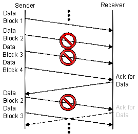
Figure 18 After Ack, when the first Data is
lost
Any packet can be lost during transfer, so there is
timeout for every wait to prevent indefinite waiting. Figure
12 shows case with no packet loss. When Open packet is
lost as in Figure 13, Open is retransmitted after timeout. When Ack for
Open is lost as in Figure 13Figure 14, Open is retransmitted also after timeout. Figure 15 shows what happens if Data packet is lost. After
looking at acknowledgement, sender resends lost data. Figure
16 shows when Ack for data is lost. Sender times out.
This is clearer in Figure 17. As shown, receiver does not timeout to send Ack.
There are two reasons why only sender times out and
stimulate receiver for Ack. The first reason is shown in Figure 16. If sender doesn’t time out, for a receiver to make
sure Ack is delivered to sender, receiver should get acknowledgement from
sender for Ack itself. This is not good. So it is clear that sender should
timeout. Given that sender times out, timeout of receiver makes no difference
except that channel is wasted by unnecessary Ack from receiver. So timeout in
only sender side is desirable. As a second reason, if receiver times out, in
case like Figure 18 (if first Data after Ack is lost), second Data always
collide with resent Ack of receiver. This is not a good phenomenon. Therefore,
after sending last packet in each round, if acknowledgement does not come,
sender sends the last packet in that round again to stimulate acknowledgement.
However, this does not mean receiver has no timeout. Receiver waits sufficient
amount of time, and if nothing happens, it regards the situation as a failure.
Figure 19 shows state transition diagram of sender, and Figure 20 shows state transition diagram of receiver.
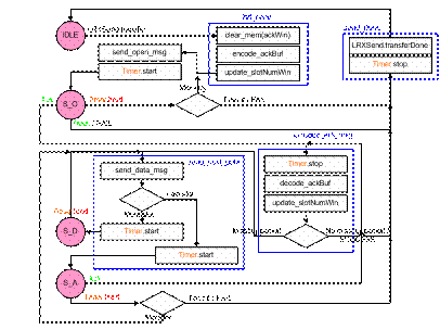
Figure 19 State Transition Diagram of Sender
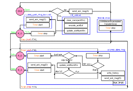
Figure 20 State Transition Diagram of Receiver
5.2.
Evaluation
Two performance metrics are evaluated: throughput,
robustness. Robustness is partially tested by looking at whether LRX
successfully works under high loss rate.
There are three factors which determine throughput:
interval between packets, window size, and loss rate.
Interval between packets is controlled by timer not
to saturate channel. Now throttle is fixed at 10 packets per second. Better way
would be throttling sending rate by looking at channel quality, like loss rate.
This issue will be discussed more in Section 8 Future Work. For tests here,
fixed rate (10 packets per second) is used.
Window size determines relative overhead of control
packets (open session, acknowledgement). Therefore, as window size increases,
throughput also increases. Figure 21 shows test result. Optimal case is when window size
is infinite. For the case with window size 16, throughput is 88% of optimal
case. Considering loss rate of 3%, actual relative throughput is 91%, which is
higher than 85% of channel utilization ratio. This is because 1) LRX tag
overhead is included for optimal case, 2) control packets do not follow 10
packets/s.
Loss rate determines overhead for retransmissions
for lost packets. As loss rate increases, retransmission increases, and throughput
decreases. Figure 22 shows the result. This graph also shows robustness of
LRX. Even with loss rate above 20%, LRX successfully transfers data.
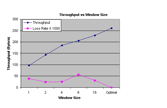
Figure 21 Throughput vs Window Size
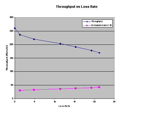
Figure 22 Throughput vs Loss Rate
Table 2 Channel Utilization
|
|
TOS_Msg |
LRX
(only data) |
LRX
(Window Size 16) |
|
Total
Data (bytes) |
36 |
36 |
613 |
|
Meta
Data (bytes) |
7 |
10 |
197 |
|
Real
Data (bytes) |
29 |
26 |
416 |
|
Channel
Utilization (%) |
78.38 |
72.22 |
67.86 |
|
Comparison
to TOS_Msg (%) |
100 |
89.66 |
84.24 |
Table 2 shows channel utilization for TOS_Msg, and data
message of LRX, and overall LRX. TOS_Msg has an overhead of 7 bytes, and LRX
data has 3 bytes overhead. Inclusion of overhead of control message further
decreases channel utilization. LRX (data only) is the theoretical limit of LRX
(when window size is infinite). We can see that using LRX lowers channel
utilization by 15%.
6.
Signal Processing and System Identification
As an analog signal processing low-pass filter is
used, which filters high frequency noise. However as shown in Figure 23, loss-pass filter is not perfect, and there exists
some leftover signal above threshold frequency. Therefore even if low-pass
filter is used, sampling frequency at ADC should be higher than threshold frequency
of low-pass filter. Moreover by Nyquist theorem, to avoid aliasing, sampling
rate should be at least twice of signal’s frequency. For accelerometer board,
low-pass filter with threshold frequency 25Hz is used. Then ADC should sample
at frequency much higher than 50Hz.
As a digital signal processing, averaging is used.
If noise follows Gaussian distribution, by averaging N numbers, noise decreases
by a factor of sqrt(N). This multiplies sampling frequency by a factor of N.
Currently averaging is optionally used for testing.

Figure 23 Imperfect Loss-pass Filter
System identification is identifying model of
target system. By matching input to system and output from system, we can
construct a mathematical system model. Usual process is fitting a general
Box-Jenkins multi-input multi-output model to sampled data. And natural
frequencies, damping ratios and mode shape are then estimated using the
estimated Box-Jenkins model. Most part of system identification is to be done
in the future.
7.
Conclusion
New challenges are analyzed which are brought by
structure monitoring to wireless sensor network. High accuracy accelerometer,
high frequency sampling with low jitter, low-pass filter, averaging,
large-scale reliable data collection, they all were not critical issues in
conventional application of wireless sensor networks. Those challenges are
overcome to sufficient degrees, however there are still many problems to be
solved.
Figure 24 shows accelerometer accuracy and diverse challenges
which will be encountered in pursuit of each degree of accuracy. It is
straightforward that to achieve higher accuracy target, we should overcome more
challenges. Those challenges in the figure are only a subset of already
recognized problems. We can expect unrecognized problems will give
additional challenges. However, as we can see in Figure
25, the extent of applications enabled also increases,
as accuracy increases.
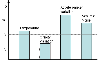
Figure 24 Challenges versus Accuracy
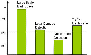
Figure 25 Possible Applications versus Accuracy
8.
Future Work
Accelerometer should be calibrated with respect to
temperature. Industry uses even 5th order polynomial for
calibration. It requires a huge amount of effort. This is not feasible in our
case. First, calibration cost is too high for low cost wireless sensor
networks. Second, computation like 5th order polynomial for each
sample is too expensive in lese powerful, low cost devices. Therefore
de-trending at server side will be a good solution. After stamping each data or
each set of data with temperature, we can process later.
Temporal jitter is handled by high frequency
sampling component. Spatial jitter should be solved by time synchronization.
ITP [8] is a time synchronization protocol widely used in Internet. In wireless
sensor network, there were several studies. In RBS [9], synchronization is done
among receivers, eliminating sender’s jitter in media access. TPSN [10] put
time stamp after obtaining channel. This gives even better synchronization
accuracy than RBS (10μs compared to 20μs). Still there is a source of
jitter at receiver side. As we saw in jitter for sampling, handling interrupt
by radio can be delayed by atomic section of other activity. As suggested in
[10], putting time stamp at MAC layer in receiver side will eliminate this
jitter.
To maximize utility of channel, we need to monitor
channel quality (loss rate), and throttle packet injection rate accordingly.
This is very like media access control, just at higher level. This requires
eavesdropping channel, and needs access to lower network layer breaking
hierarchy.
LRX transfers data from RAM to RAM. Using LRX as a
building block, multi-hop data collection need be implemented. Exploiting
linear geography of bridge, pipelining can be used. Multi-channel can
distribute traffic over multiple frequency spectrum and increase throughput.
Supernode like Stargate can be also used.
As a digital signal process, digital low-pass
filter can be used, to eliminate effect of imperfect analog low-pass filter.
9.
Acknowledgement
This work is a part of ‘Structural Health
Monitoring of the
10.
Reference
[1]
Philo Juang, Hide Oki, Yong Wang, Margaret Martonosi, Li-Shiuan Peh, Daniel
Rubenstein. Energy-Efficient Computing for Wildlife Tracking: Design Tradeoffs
and Early Experiences with ZebraNet, in Proceedings of ASPLOS-X,
[2]
Alan Mainwaring, Joseph Polastre, Robert Szewczyk, David Culler, John Anderson.
Wireless Sensor Networks for Habitat Monitoring, in the 2002 ACM International
Workshop on Wireless Sensor Networks and Applications. WSNA '02,
[3]
Clement Ogaja, Chris Rizos, Jinling Wang, James Brownjohn. Toward the
Implementation of On-line Structural Monitoring Using RTK-GPS and Analysis of
Results Using the Wavelet Transform.
[4]
Penggen Cheng, Wenzhong John Shi, Wanxing Zheng. Large Structure Health Dynamic
Monitoring Using GPS Technology.
[5]
Juan M. Caicedo, Johannio Marulanda, Peter Thomson, and Shirley J. Dyke.
Monitoring of Bridges to Detect Changes in Structural Health, in the
Proceedings of the 2001 American Control Conference,
[6]
Jerome Peter Lynch, Anne S. Kiremidjian, Kincho H. Law, Thomas Kenny and Ed
Carryer. Issues in Wireless Structural Damage Monitoring Technologies, in the
Proceedings of the 3rd World Conference on Structural Control (WCSC),
[7]
http://webs.cs.berkeley.edu/tos/hardware/hardware.html
[8]
Mills, D.L. Internet time synchronization: the Network Time Protocol. IEEE
Trans. Communications 39, 10 (October 1991), 1482-1493.
[9]
Jeremy Elson, Lewis Girod and Deborah Estrin. Fine-Grained Network Time
Synchronization using Reference Broadcasts, in Proceedings of the Fifth
Symposium on Operating Systems Design
and
Implementation (OSDI 2002),
[10]
Saurabh Ganeriwal, Ram Kumar, Mani B. Srivastava. Timing-Sync protocol for
Sensor Networks, in SenSys ’03,